PostgreSQL as a Graph Database: Who Grabbed a Beer Together?
27 Dec 2025Graph databases have become increasingly popular for modeling complex relationships in data. But what if you could leverage graph capabilities within the familiar PostgreSQL environment you already know and love? In this article, I’ll explore how PostgreSQL can serve as a graph database using the Apache AGE extension, demonstrated through a fun use case: analyzing social connections in the craft beer community using Untappd data.
This article is based on my presentation at PgConf.EU 2025 in Riga, Latvia. Special thanks to Pavlo Golub, my co-founder of the PostgreSQL Ukraine community, whose Untappd account served as the perfect example for this demonstration.
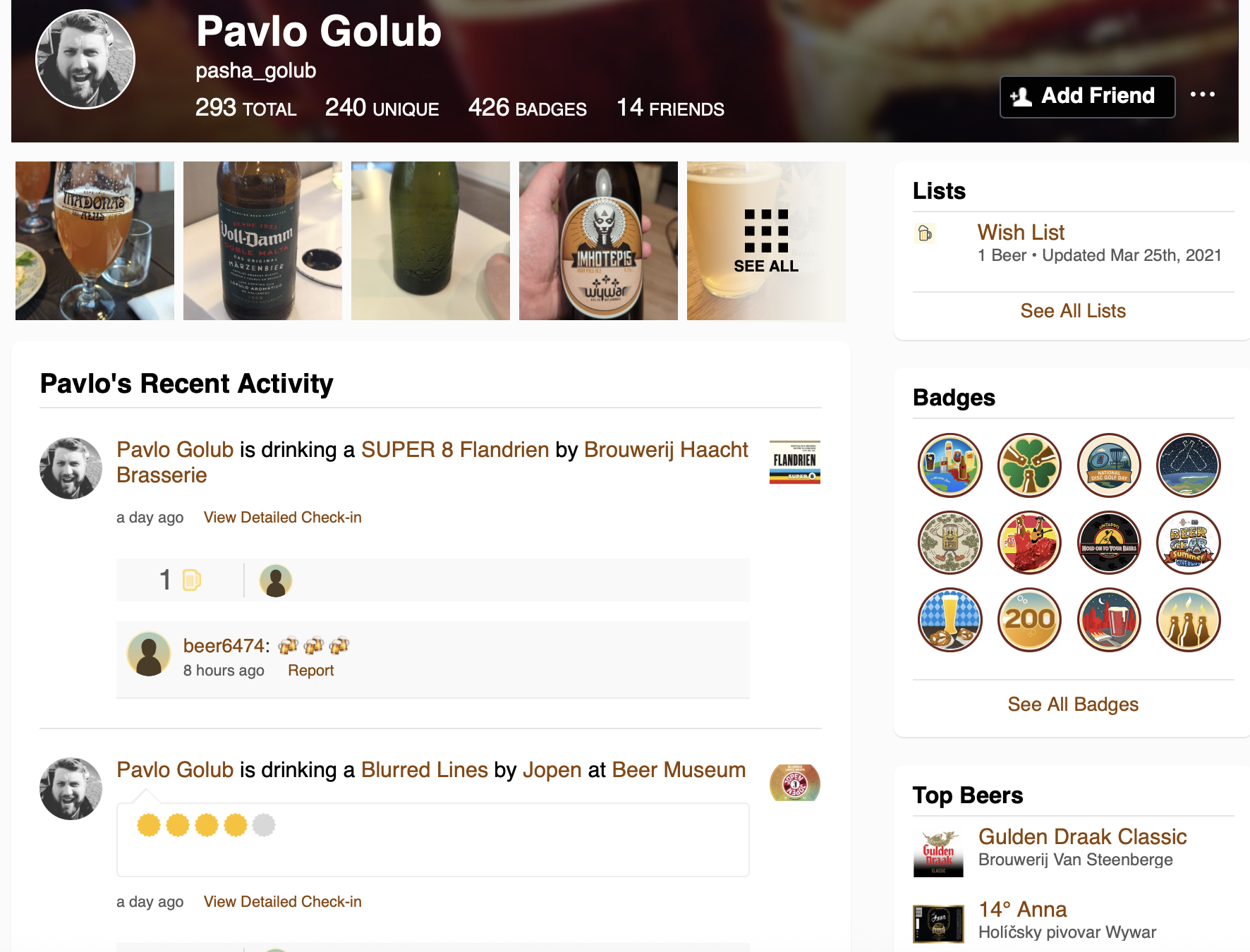 Pavlo Golub’s Untappd profile - the starting point for our graph analysis
Why Graph Databases?
Traditional relational databases excel at storing structured data in tables, but they can struggle when dealing with highly interconnected data. Consider a social network where you want to find the shortest path between two users through their mutual connections—this requires recursive queries with CTEs, joining multiple tables, and becomes increasingly complex as the depth of relationships grows.
You might say: “But I can do this with relational tables!” And yes, you would be right in some cases. But graphs offer a different approach that makes certain operations much more intuitive and efficient.
Graph databases model data as nodes (vertices) and edges (relationships), making them ideal for:
- Social networks
- Recommendation engines
- Fraud detection
- Knowledge graphs
- Network topology analysis
Basic Terms in Graph Theory
Before diving into implementation, let’s establish some fundamental concepts:
Vertices (Nodes) are the fundamental units or points in a graph. You can think of them like tables in relational databases. They represent entities, objects, or data items—for example, individuals in a social network.
Edges (Links/Relationships) are the connections between nodes that indicate relationships. These are the links between your vertices. They can be directed or undirected and may have weights or properties.
Graph is a collection of vertices and edges forming a structure. When you bring vertices and edges together, they create your graph.
Path is a sequence of edges connecting two nodes. If you want to connect some vertices and need to pass through multiple nodes, this becomes your path.
Degree is the number of edges connected to a node. Your node can have different connections, and the count of these connections describes its degree.
The Untappd Use Case
When you want to demonstrate something, you need real data. Untappd is a social networking platform for craft beer enthusiasts that provides a perfect example. Users can check in beers they’re drinking, rate them, add photos, and interact with friends.
The platform exposes rich social data through user profiles and activity feeds, including:
- Full name and username
- Friends list
- Check-ins with beer, brewery, venue, rating, timestamp
- Comments on check-ins
- Toasts (likes) on check-ins
- Photos shared
In a traditional relational approach, this data would be modeled with separate tables connected by foreign keys:
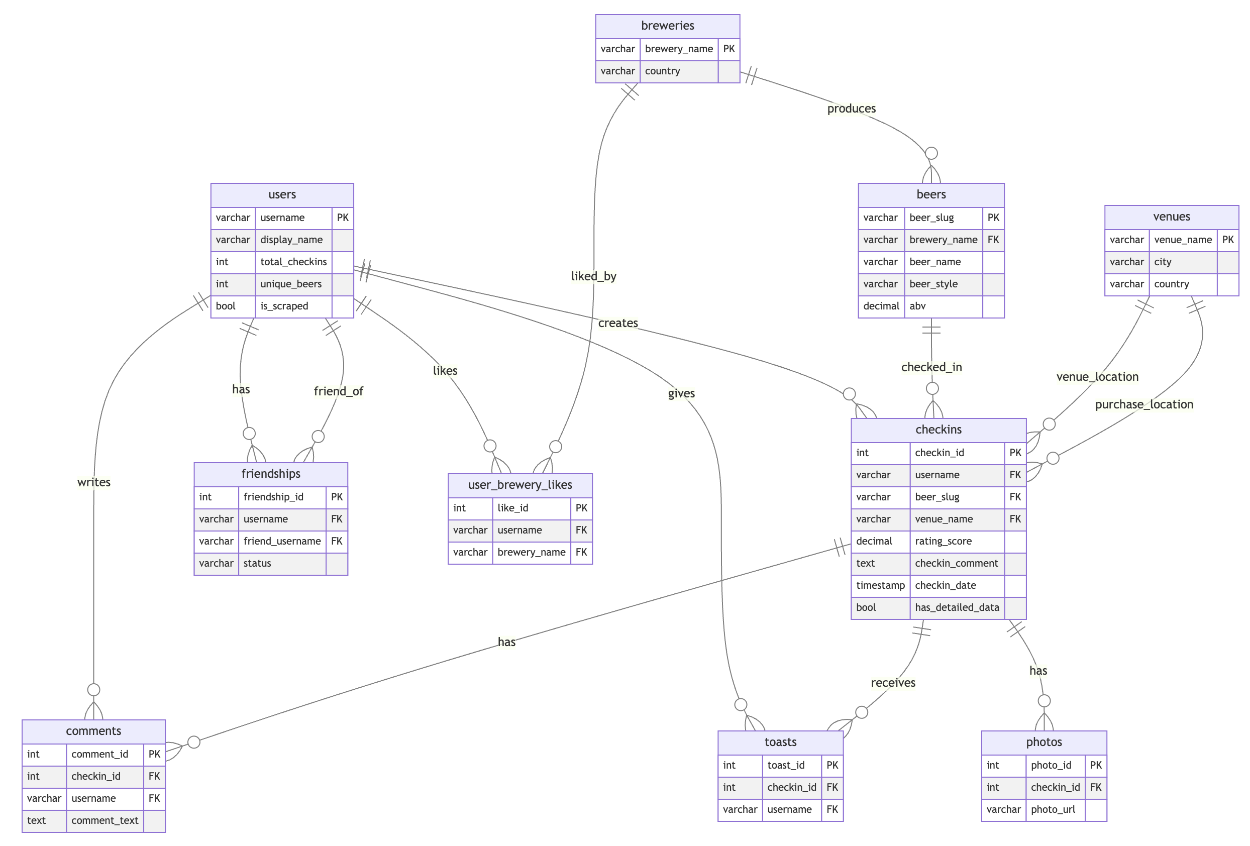 Traditional relational schema for Untappd data
This data naturally forms a graph where we might want to answer questions like: “What’s the shortest path between two users?” or “Who grabbed a beer together?”
The Graph Model
Instead of the relational model with separate tables for users, breweries, beers, venues, and check-ins with foreign key relationships, we can model the same data as a graph:
Node Types:
User (username)
Checkin (checkin_id, rating, serving_style, comment, date, photos)
Beer (beer_slug)
Brewery (brewery_name)
Venue (venue_name)
Relationships (Edges):
User -[FRIEND_OF {status}]-> User
User -[CHECKED_IN]-> Checkin
User -[TOASTED]-> Checkin
User -[COMMENTED {text, timestamp}]-> Checkin
User -[WISHLIST]-> Beer
User -[LIKES_BREWERY]-> Brewery
Checkin -[FOR_BEER]-> Beer
Checkin -[AT_VENUE]-> Venue
Checkin -[PURCHASED_AT]-> Venue
Beer -[BREWED_BY]-> Brewery
 Graph model showing nodes and relationships in the Untappd data
Here’s how you would create this graph model in Apache AGE using Cypher:
-- Create the graph
SELECT create_graph('untappd_graph');

-- Create nodes
SELECT * FROM cypher('untappd_graph', $$
  CREATE (u:User {username: 'taras', name: 'Taras Kloba'})
  CREATE (b:Beer {beer_slug: 'guinness-draught', name: 'Guinness Draught'})
  CREATE (br:Brewery {brewery_name: 'guinness', name: 'Guinness'})
  CREATE (v:Venue {venue_name: 'irish-pub-kyiv', name: 'Irish Pub Kyiv'})
  CREATE (c:Checkin {checkin_id: 1, rating: 4.5, date: '2024-12-27'})
$$) AS (result agtype);

-- Create relationships
SELECT * FROM cypher('untappd_graph', $$
  MATCH (u:User {username: 'taras'}), (c:Checkin {checkin_id: 1})
  CREATE (u)-[:CHECKED_IN]->(c)
$$) AS (result agtype);

SELECT * FROM cypher('untappd_graph', $$
  MATCH (c:Checkin {checkin_id: 1}), (b:Beer {beer_slug: 'guinness-draught'})
  CREATE (c)-[:FOR_BEER]->(b)
$$) AS (result agtype);

SELECT * FROM cypher('untappd_graph', $$
  MATCH (c:Checkin {checkin_id: 1}), (v:Venue {venue_name: 'irish-pub-kyiv'})
  CREATE (c)-[:AT_VENUE]->(v)
$$) AS (result agtype);

SELECT * FROM cypher('untappd_graph', $$
  MATCH (b:Beer {beer_slug: 'guinness-draught'}), (br:Brewery {brewery_name: 'guinness'})
  CREATE (b)-[:BREWED_BY]->(br)
$$) AS (result agtype);
The visualization of this data becomes quite impressive when you can navigate through thousands of connections and see relationships that would be difficult to discover in tabular data.
Finding Paths: SQL vs Cypher
Imagine you want to find the closest path between two users. They can have different interactions between them—comments, toasts (likes), friendships, liking the same beer or brewery. There are many possible ways to find connections between two users.
The SQL Approach (Recursive CTE)
With regular SQL, this becomes quite challenging. You need recursive queries with CTEs, going through all the relationship tables, finding users in one table, trying to find connections to other users:
WITH RECURSIVE
-- Build a unified graph of all user connections
user_connections AS (
    -- Direct friendships (bidirectional)
    SELECT   username AS user1,
             friend_username AS user2,
             'friendship' AS connection_type,
             1 AS weight
    FROM     friendships
    WHERE    status = 'active'

    UNION ALL

    SELECT   friend_username AS user1,
             username AS user2,
             'friendship' AS connection_type,
             1 AS weight
    FROM     friendships
    WHERE    status = 'active'

    UNION ALL

    -- Toast interactions
    SELECT DISTINCT
             t.username AS user1,
             c.username AS user2,
             'toast' AS connection_type,
             2 AS weight
    FROM     toasts t
    JOIN     checkins c ON t.checkin_id = c.checkin_id
    WHERE    t.username != c.username
    -- ... more connection types ...
),

-- Aggregate connections to find strongest link between users
aggregated_connections AS (
    SELECT   user1,
             user2,
             MIN(weight) AS min_weight,
             array_agg(DISTINCT connection_type) AS connection_types
    FROM     user_connections
    GROUP BY user1, user2
),

-- Recursive pathfinding using BFS
path_search AS (
    -- Base case: start from source user
    SELECT   :source_user::VARCHAR AS current_user,
             :source_user::VARCHAR AS path_text,
             ARRAY[:source_user::VARCHAR] AS path_array,
             0 AS total_weight,
             0 AS hop_count

    UNION ALL

    -- Recursive case: explore neighbors
    SELECT   ac.user2,
             ps.path_text || ' -> ' || ac.user2,
             ps.path_array || ac.user2,
             ps.total_weight + ac.min_weight,
             ps.hop_count + 1
    FROM     path_search ps
    JOIN     aggregated_connections ac ON ps.current_user = ac.user1
    WHERE    NOT (ac.user2 = ANY(ps.path_array))  -- Avoid cycles
      AND    ps.hop_count < 6                      -- Limit depth
      AND    ps.current_user != :target_user       -- Stop at target
)

-- Find shortest paths to target
SELECT   path_text,
         total_weight,
         hop_count AS degrees_of_separation
FROM     path_search
WHERE    current_user = :target_user
ORDER BY total_weight, hop_count
LIMIT    10;
This query is complex, verbose, and difficult to maintain.
The Cypher Approach (Apache AGE)
With Apache AGE and the openCypher syntax, the same query becomes remarkably simple:
SELECT *
FROM   cypher('untappd_graph', $$
           MATCH path = (u1:User {username: 'user1'})-[*]-(u2:User {username: 'user2'})
           RETURN nodes(path) AS all_nodes, length(path) AS hops
       $$) AS (all_nodes agtype, hops agtype)
ORDER BY hops
LIMIT  1;
With this simple line, we identify all paths that can connect two users,
calculate the number of hops between them, and then—here’s the beauty
of combining SQL with openCypher—we can use familiar operators like
ORDER BY and LIMIT to get just the shortest path.
The pattern matching syntax (u1:User)-[*]-(u2:User) naturally expresses
“find any path between two users through any edges.”
What is Apache AGE?
Apache AGE (A Graph Extension) brings native graph database capabilities to PostgreSQL. What makes it special:
openCypher Standard: This is the standard syntax for graph databases. If you’ve worked with Neo4j, you’ll find the same syntax here. This is wonderful because you can start working with one database but easily migrate to PostgreSQL and continue your work with the functionality you already know.
Part of Apache Software Foundation: When a project is part of Apache, you know they won’t suddenly stop development or abandon the project without notice. It’s also about peer reviews and sharing best practices.
Hybrid Querying: Seamlessly mix SQL and Cypher in the same query. You can wrap your Cypher query in a function, and then apply all the SQL operators you know—joins, limits, orders, aggregations—to the graph output.
How AGE Stores Data Internally
One question that often comes up: how does AGE store graph data?
The answer is elegant: everything is stored in regular PostgreSQL tables. For each vertex label, you get a table with two columns:
id: A unique identifier (sequence)properties: A JSONB column containing all the node properties
For edges, you get a table with:
id: Unique edge identifierstart_id: Reference to the source vertexend_id: Reference to the target vertexproperties: JSONB column for edge properties
This means you can query graph data with regular SQL if you prefer:
-- Query vertices with regular SQL
SELECT * FROM demo_graph."User";
Result:
| id | properties |
|---|---|
| 844424930131969 | {"city": "Lviv", "username": "Taras"} |
| 844424930131970 | {"city": "Kropyvnytskyi", "username": "Pavlo"} |
| 844424930131971 | {"city": "Stockholm", "username": "Magnus"} |
Similarly, you can query the edges table to see the relationships:
-- Query edges with regular SQL
SELECT * FROM demo_graph."FRIENDS";
Result:
| id | start_id | end_id | properties |
|---|---|---|---|
| 1125899906842625 | 844424930131969 | 844424930131970 | {"since": "2019-01-22"} |
| 1125899906842626 | 844424930131970 | 844424930131971 | {} |
Performance Optimization
Because the data is stored in regular PostgreSQL tables, you can use all the performance techniques you already know:
- Create indexes on the ID columns
- Use conditional indexes based on your query patterns
- Apply all standard PostgreSQL optimization techniques
-- Create an index on vertex properties
CREATE INDEX idx_user_username
    ON demo_graph."User"
    USING GIN ((properties -> 'username'));

-- Create a conditional index for active friendships
CREATE INDEX idx_friends_active
    ON demo_graph."FRIENDS"
    USING BTREE (start_id, end_id)
    WHERE (properties -> 'status')::TEXT = '"active"';
The query planner takes these indexes into account during optimization, just like with any other PostgreSQL query.
Apache AGE vs pgRouting
When considering graph capabilities in PostgreSQL, two main extensions stand out:
| Feature | Apache AGE | pgRouting |
|---|---|---|
| Primary Use Case | Property-graph querying | Routing and network analysis on spatial data |
| Query Language | SQL + openCypher | SQL functions |
| Data Model | Property graph over PostgreSQL tables | Relational tables with spatial topology |
| Integration | Standard PG tooling; optional AGE Viewer | GIS toolchain: PostGIS, osm2pgrouting |
| License | Apache-2.0 | GPL-2.0 |
| Azure Availability | Yes, on Azure Database for PostgreSQL | Yes, with PostGIS |
| Best For | Pattern matching, relationship queries | Shortest paths, isochrones, vehicle routing |
If you’re doing geoanalytics and have routing data, that’s also a kind of graph data, and pgRouting with PostGIS is excellent for that use case. But for general property-graph queries with openCypher syntax, Apache AGE is the way to go.
Interactive Tutorial: Getting Started
Let me walk you through a hands-on tutorial that I demonstrated live at PgConf.EU.
Step 1: Install the Extension
-- Install the AGE extension
CREATE EXTENSION IF NOT EXISTS age;

-- Configure the search path (optional but convenient)
-- All AGE functions live in the ag_catalog schema
SET search_path = ag_catalog, "$user", public;
Step 2: Create a Graph
-- Create a new graph
SELECT create_graph('demo_graph');

-- Verify in the internal catalog
SELECT * FROM ag_graph;
Result:
| graphid | name | namespace |
|---|---|---|
| 43158 | demo_graph | demo_graph |
Every graph you create is registered in the ag_graph internal table.
Step 3: Understand Labels
-- View default labels created for your graph
SELECT   l.*
FROM     ag_label l
JOIN     ag_graph g ON l.graph = g.graphid
WHERE    g.name = 'demo_graph';
Result:
| name | graph | id | kind | relation | seq_name |
|---|---|---|---|---|---|
| _ag_label_vertex | 43158 | 1 | v | demo_graph._ag_label_vertex | _ag_label_vertex_id_seq |
| _ag_label_edge | 43158 | 2 | e | demo_graph._ag_label_edge | _ag_label_edge_id_seq |
Every graph starts with two default labels: one for vertices (_ag_label_vertex) and one for edges (_ag_label_edge).
Step 4: Create a Vertex Label
-- Create a label for Users (this creates a PostgreSQL table)
SELECT create_vlabel('demo_graph', 'User');
This physically creates a new table demo_graph."User" to store User
vertices.
Step 5: Create Nodes
-- Create first user: Taras from Lviv
SELECT *
FROM   cypher('demo_graph', $$
           CREATE (u:User {username: 'Taras', city: 'Lviv'})
           RETURN u
       $$) AS (u agtype);
Result:
| u |
|---|
{"id": 844424930131969, "label": "User", "properties": {"city": "Lviv", "username": "Taras"}}::vertex |
-- Create second user: Pavlo from Kropyvnytskyi
SELECT *
FROM   cypher('demo_graph', $$
           CREATE (u:User {username: 'Pavlo', city: 'Kropyvnytskyi'})
           RETURN u
       $$) AS (u agtype);
Result:
| u |
|---|
{"id": 844424930131970, "label": "User", "properties": {"city": "Kropyvnytskyi", "username": "Pavlo"}}::vertex |
Each vertex gets a unique ID automatically.
Step 6: Query with SQL and Cypher
-- Regular SQL query
SELECT * FROM demo_graph."User";
Result (SQL):
| id | properties |
|---|---|
| 844424930131969 | {"city": "Lviv", "username": "Taras"} |
| 844424930131970 | {"city": "Kropyvnytskyi", "username": "Pavlo"} |
-- Same data with Cypher
SELECT *
FROM   cypher('demo_graph', $$
           MATCH (u:User)
           RETURN u.username, u.city
       $$) AS (username agtype, city agtype);
Result (Cypher):
| username | city |
|---|---|
| “Taras” | “Lviv” |
| “Pavlo” | “Kropyvnytskyi” |
Step 7: Create Relationships
-- Create FRIENDS relationship between Taras and Pavlo
SELECT *
FROM   cypher('demo_graph', $$
           MATCH  (taras:User {username: 'Taras'}),
                  (pavlo:User {username: 'Pavlo'})
           CREATE (taras)-[r:FRIENDS {since: '2019-01-22'}]->(pavlo)
           RETURN r
       $$) AS (friendship agtype);
The edge contains start_id and end_id referencing our vertices (69
and 70), plus the properties we defined.
Note: The FRIENDS edge label was created automatically—AGE handles this for you when you first use a new edge type.
Step 8: Create User and Relationship Together
-- Create Magnus and connect to Pavlo in one command
SELECT *
FROM   cypher('demo_graph', $$
           MATCH  (pavlo:User {username: 'Pavlo'})
           CREATE (pavlo)-[:FRIENDS]->(:User {username: 'Magnus', city: 'Stockholm'})
       $$) AS (result agtype);
Step 9: Build a Network with Multiple Paths
Let’s expand our graph by adding more users and creating connections between them to form a network with multiple possible paths:
-- Add more users
SELECT *
FROM   cypher('demo_graph', $$
           CREATE (u1:User {username: 'Olena', city: 'Odesa'}),
                  (u2:User {username: 'Ivan', city: 'Kharkiv'})
           RETURN u1.username, u2.username
       $$) AS (user1 agtype, user2 agtype);

-- Create connection: Magnus -> Olena
SELECT *
FROM   cypher('demo_graph', $$
           MATCH  (magnus:User {username: 'Magnus'}),
                  (olena:User {username: 'Olena'})
           CREATE (magnus)-[:FRIENDS]->(olena)
       $$) AS (result agtype);

-- Create connection: Olena -> Ivan
SELECT *
FROM   cypher('demo_graph', $$
           MATCH  (olena:User {username: 'Olena'}),
                  (ivan:User {username: 'Ivan'})
           CREATE (olena)-[:FRIENDS]->(ivan)
       $$) AS (result agtype);

-- Create alternative path: Taras -> Ivan (direct)
SELECT *
FROM   cypher('demo_graph', $$
           MATCH  (taras:User {username: 'Taras'}),
                  (ivan:User {username: 'Ivan'})
           CREATE (taras)-[:FRIENDS]->(ivan)
       $$) AS (result agtype);
Now we have a network with multiple paths:
Taras -> Pavlo -> Magnus -> Olena -> Ivan (4 hops)
Taras -> Ivan (1 hop, direct)
Step 10: Query Users and Friends
Now let’s query the graph to see each user with their list of friends using Cypher’s collect() aggregation function:
-- Use aggregation to collect friends into an array
SELECT *
FROM   cypher('demo_graph', $$
           MATCH  (u:User)-[r:FRIENDS]-(friend:User)
           RETURN u.username, collect(friend.username) AS friends
       $$) AS (username agtype, friends agtype);
Result:
| username | friends |
|---|---|
| “Ivan” | ["Olena", "Taras"] |
| “Magnus” | ["Olena", "Pavlo"] |
| “Olena” | ["Magnus", "Ivan"] |
| “Pavlo” | ["Taras", "Magnus"] |
| “Taras” | ["Ivan", "Pavlo"] |
Step 11: Find Shortest Path
One of the most powerful graph operations is finding the shortest path between two nodes. Here’s how to find the shortest path from Taras to Magnus:
-- Find shortest path from Taras to Magnus
SELECT   *
FROM     cypher('demo_graph', $$
             MATCH path = (u1:User {username: 'Taras'})-[*]-(u2:User {username: 'Magnus'})
             RETURN path, length(path) AS hops
         $$) AS (path agtype, hops agtype)
ORDER BY hops
LIMIT    1;
Result:
| path | hops |
|---|---|
Taras -[FRIENDS]-> Pavlo -[FRIENDS]-> Magnus |
2 |
The path shows: Taras → Pavlo → Magnus (2 hops)
Step 12: Find All Paths
We can also find all possible paths between two users, not just the shortest one. By removing the LIMIT 1 and adding a length constraint, we can discover alternative routes:
-- Find ALL paths up to 5 hops
SELECT   *
FROM     cypher('demo_graph', $$
             MATCH path = (u1:User {username: 'Taras'})-[*]-(u2:User {username: 'Magnus'})
             WHERE length(path) <= 5
             RETURN path, length(path) AS hops
         $$) AS (path agtype, hops agtype)
ORDER BY hops;
Result:
| path | hops |
|---|---|
Taras -[FRIENDS]-> Pavlo -[FRIENDS]-> Magnus |
2 |
Taras -[FRIENDS]-> Ivan <-[FRIENDS]- Olena <-[FRIENDS]- Magnus |
3 |
This shows both paths:
- Short path (2 hops): Taras → Pavlo → Magnus
- Alternative path (3 hops): Taras → Ivan ← Olena ← Magnus
Step 13: Clean Up
When you’re done experimenting, you can remove the graph and all its associated tables with a single command:
-- Drop the graph (cascade deletes all internal tables)
SELECT drop_graph('demo_graph', true);
Who’s Grabbing a Beer in the PostgreSQL Community?
To answer our original question, I identified Untappd accounts of speakers at PostgreSQL conferences and collected information about their interactions. The visualization reveals fascinating patterns:
-
Community hubs: Some people have many connections and are at the “heart” of the community. By such activities, you can get closer to the center of the community.
-
Separate clusters: Some speakers participate in conferences but their Untappd connections are primarily with other communities, not the PostgreSQL community. This is visible as distant clusters in the 3D visualization.
-
Connection patterns: You can identify who frequently checks in at the same venues during conferences, suggesting they grabbed beers together.
The visualization uses react-graph-force, a React library for 3D graph visualization. While 3D graphs are more common in biotechnology and scientific analysis, they provide unique insights for community analysis too.
A Note on Responsible Data Sharing
During this analysis, I noticed something important: people share photos on social media without realizing what’s visible in the background.
I found photos where:
- Conference badges with full names were clearly readable
- Laptop screens showed sensitive information
- Sticky notes with what appeared to be credentials were visible
Think about what you share on the internet. What seems like an innocent beer photo might reveal more than you intended.
Conclusion
PostgreSQL’s extensibility makes it a powerful platform for graph database capabilities through Apache AGE. If your application requires both relational and graph queries, or if you want to add graph capabilities without introducing a new database technology to your stack, Apache AGE is worth exploring.
The key advantages:
- Familiar infrastructure: Use your existing PostgreSQL expertise, tools, monitoring, and backup solutions
- Standard syntax: openCypher compatibility means easy migration from other graph databases
- Hybrid queries: Combine graph pattern matching with SQL analytics
- Performance tuning: Use standard PostgreSQL indexing and optimization techniques
Whether you’re analyzing who grabbed a beer together, building a recommendation engine, or detecting fraud patterns, PostgreSQL with Apache AGE provides a compelling solution.
Additional Resources
- Apache AGE Official Documentation
- Apache AGE GitHub Repository
- openCypher Specification
- AGE Viewer - Visual graph exploration tool
- react-graph-force - 3D graph visualization
- Azure Database for PostgreSQL - Managed PostgreSQL with AGE support
This article is based on my presentation “PostgreSQL as a Graph Database: Who Grabbed a Beer Together?” delivered at PgConf.EU 2025 in Riga, Latvia.